How to Use Pivot Tables in Google Sheets: Full Guide

You have a sheet with 1,000 rows of sales data. Your manager asks: "How much did each region bring in last quarter?" You could write a bunch of SUMIF formulas... or you could build a pivot table in 30 seconds and have the answer.

Pivot tables are the most powerful feature most Google Sheets users never learn. This guide shows you exactly how to use pivot tables in Google Sheets — from inserting your first one to customizing it for real analysis.

What Is a Pivot Table in Google Sheets?

A pivot table is a tool that automatically summarizes large datasets. You tell it which columns to group by, which values to calculate, and it does the math — no formulas needed.

For example: if you have a spreadsheet with 1,000 rows of orders (each with a product, region, date, and amount), a pivot table can instantly show you total sales by product, total orders by region, or average order value by month.

The name comes from "pivoting" data — you can rearrange how data is grouped with a few clicks, turning rows into columns and vice versa.

When to use pivot tables:

• Summarizing sales, expenses, or usage data
• Counting occurrences across categories
• Comparing performance across groups
• Finding totals, averages, or counts without writing formulas

What You Will Need

• A Google account with Google Sheets access
• A spreadsheet with at least one column of categories and one column of numbers
• Data with headers in the first row — no merged cells, no gaps

The dataset does not need to be huge. Pivot tables work with 50 rows just as well as 50,000.

Step-by-Step: How to Use Pivot Tables in Google Sheets

Step 1: Prepare Your Data

Before inserting a pivot table, make sure your data is clean:

• Row 1 is headers — every column needs a name (Region, Product, Amount, Date, etc.)
• No merged cells in the data range
• No completely empty rows in the middle of the data
• Consistent data types — don't mix text and numbers in the same column

If your data has any of these issues, fix them first. Pivot tables can handle messy data, but the results will be confusing.

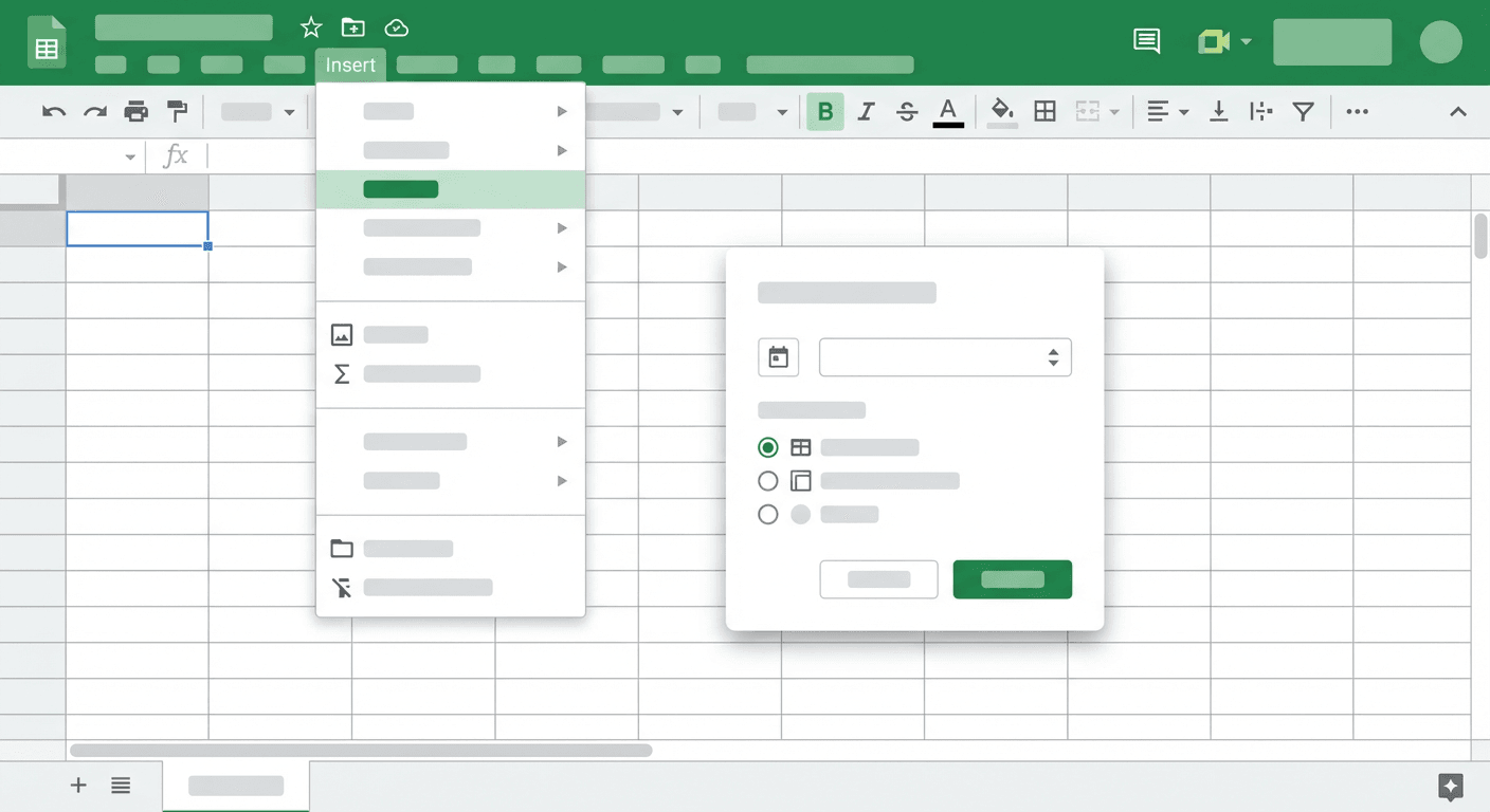
Step 2: Insert a Pivot Table

1. Click any cell inside your data range
2. Go to Insert → Pivot table
3. A dialog appears asking where to put it:
   • New sheet (recommended) — keeps the pivot table separate from your raw data
   • Existing sheet — lets you specify a cell location
4. Click Create

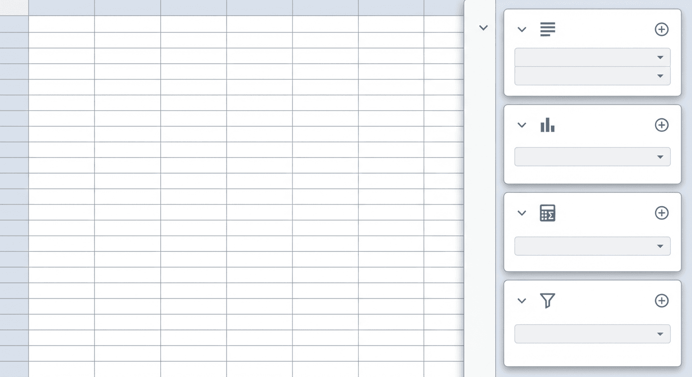
Google Sheets opens a new sheet with an empty pivot table grid and a Pivot table editor panel on the right.

Step 3: Add Rows

In the Pivot table editor panel, click Add next to Rows. Select the column you want to group by.

If you select "Region", each row in the pivot table becomes a region. If you select "Product", each row becomes a product.

You can add multiple row fields — they nest. Adding "Region" then "Product" shows products grouped inside each region.

Step 4: Add Values

Click Add next to Values. Select the column you want to calculate.

By default, Google Sheets will SUM numeric columns. Click the value field to choose a different summary type:

• SUM — total of all values in the group
• COUNT — number of rows in the group
• AVERAGE — mean value
• MAX / MIN — highest or lowest value
• COUNTUNIQUE — number of distinct values

This is where pivot tables save hours of SUMIF and COUNTIF formulas.

Step 5: Add Columns (Optional)

Click Add next to Columns to create a cross-tab view. Example: rows = Region, columns = Quarter, values = SUM of Amount. You get a table showing sales per region per quarter in a single view.

Step 6: Add Filters (Optional)

Click Add next to Filters to limit what data appears in the pivot table. This is useful for:

• Showing only one time period (filter by year or quarter)
• Excluding cancelled orders (filter by status)
• Focusing on specific products or categories

Filters don't delete data — they just hide rows that don't match.

Step 7: Sort and Display Options

Click on any row or value field in the editor to sort. You can:

• Sort rows by value (show the highest-selling region first)
• Show or hide grand totals using the toggle in each field's settings
• Show values as percentages of the total

Your pivot table updates instantly as you make changes — no recalculating, no waiting.

Pivot Table Tips and Best Practices

A few things that make pivot tables much more useful:

Keep raw data in its own sheet. Build your pivot tables on separate sheets. If you edit raw data, the pivot table updates automatically — but only if your data range includes the new rows. Use an open-ended range (like A:F instead of A1:F500) to include future rows automatically.

Use calculated fields for custom math. In the Values section, click the drop-down on any value and choose Add calculated field. This lets you write a formula using other columns — for example, calculating profit margin directly inside the pivot table without adding new columns to your source data.

Group dates by month or quarter. If you're grouping by a date column, right-click a date value in the pivot table and choose Create pivot date group → select Month, Quarter, or Year. Google Sheets groups by day by default, which makes date-heavy data unreadable.

Refresh after data changes. Google Sheets pivot tables update automatically in most cases, but after large data imports, right-click the pivot table and choose Refresh to force an update.

Duplicate before experimenting. Pivot tables are fast to build but easy to accidentally reconfigure. Duplicate the sheet before making big structural changes — it's faster than undoing a series of mistakes.

Common Mistakes to Avoid

Merged cells in source data. Merged cells break pivot tables. Unmerge everything in your data range before inserting. Select the range, go to Format → Merge cells → Unmerge.

Fixed data ranges that miss new rows. If you defined your range as A1:F500 and later add row 501, the pivot table won't include it. Use A:F (entire columns) instead.

Pivot tables and raw data on the same sheet. This gets messy fast. One sheet for data, one sheet per pivot table — especially in shared spreadsheets where teammates might accidentally edit the pivot table itself.

Expecting live external data. Pivot tables only work with data inside the same spreadsheet. If your data lives in a database, CRM, or another tool, you need to import it first. For live external data, consider building a dashboard with a real YouBase data connection instead.

Beyond Pivot Tables: Build a Live Dashboard with YouWare

Pivot tables are great for you. They're not great for sharing with people who don't live in spreadsheets.

If you need to share analysis with teammates who aren't spreadsheet-savvy — or if you want a dashboard that looks polished and updates from live data — that's where YouWare comes in.

YouWare is a Vibe Coding platform: describe the dashboard you want in plain English, and AI builds it as a real web app. No HTML, no JavaScript, no hosting setup.

You could say: "Build a sales dashboard that reads from my Google Sheet and shows revenue by region as a bar chart, with a dropdown to filter by quarter." YouWare builds it. You get a shareable URL that anyone on your team can open in a browser — no spreadsheet access, no pivot table knowledge required.

The same data that powers your pivot table can power a web dashboard that the whole team can actually use.

FAQ

Conclusion

Pivot tables are the fastest way to summarize data in Google Sheets. Once you've built one, you'll wonder how you survived with manual SUMIF formulas.

The key steps: clean your data → Insert → Pivot table → add Rows and Values → add Columns and Filters as needed. The whole thing takes under five minutes once you know what you're doing.

And when you're ready to share that analysis as something more polished than a spreadsheet — a live dashboard, a web app your whole team can access — YouWare can build it from your Google Sheets data in minutes.